MLTC使用指南
MLTC概述
MLTC(Multi-Level Tensor Compiler)是基于MLIR研发的端到端深度学习编译器,可以将来自不同框架的AI模型编译为适配硬件产品的可执行文件,同时加速AI模型的计算过程,提高系统的健壮性。
MLTC具有以下特性:
-
通过多层IR设计实现逐层下降 ,解决代码生成的复杂性。每次IR层级的转换只专注代码生成的一个局部方面,例如多核执行模型、bufferization、算子逻辑的指令组合等。
-
提供一套算子无关的tiling系统,把一些算子的公共逻辑提升到编译器框架中,减轻算子编程的开发负担,提高系统的健壮性。面向NeuralScale架构编写算子时,不管是手写算子还是compute/schedule的DSL描述,其中大部分代码逻辑是管理多层存储结构和其间的数据传输。
-
性能优化以独立的优化pass形式作用在特定层级的IR上,可以任意打开或关闭,不影响系统健壮性。
-
保持图优化之后的编译器主干流程与算子无关,不存在任何针对特定算子的定制化逻辑。
-
保持图层IR算子的原子性,不包含可以由简单算子组合而成的复杂算子,没有融合算子。
前提条件
准备好模型推理环境,安装HPE、MLTC、Python 3.10。具体操作,请参见STCRP安装指南。
在NPU上部署模型
TensorFlow模型
部署TensorFlow模型时,需先通过MLTC的前端转换工具处理模型,再调用MLTC的编译与部署接口完成编译和部署。
-
调用MLTC的
TfToStc().run接口解析AI框架导出的模型文件,转换为MLTC自定义的图层IR。接口需要指定输入输出文件路径,和输入节点。示例参考:TfToStc().run("deepfm.pb", "deepfm_stc.mlir", "feat_index:1024x39xi32,feat_value:1024x39xf32 -s", "Sigmoid") -
调用MLTC的
Compiler().compile接口编译模型,将转换得到的MLIR文件编译为在目标设备上部署的vmfb文件。接口需要指定输入输出文件路径,支持编译参数控制编译过程。Compiler().compile("deepfm_stc.mlir", "deepfm.vmfb", "-arch=npu-v1 --dump-ir-after-all") -
调用MLTC的
Executor().run()接口部署模型,将编译得到的vmfb文件部署到NPU板卡上。接口需要指定输入的vmfb文件路径以及输入数据文件。Executor("deepfm.vmfb").run(input_data)
说明:具体Python接口定义请参见Python API。
具体可参考DeepFM模型的实现示例:
import os
import numpy as np
from mltc import Compiler
from mltc import TfToStc
from mltc import Executor

def gen_fake_data(input_shapes, input_dtype, low=0, high=2):
    input_data = {}
    for (name, shape), dtype in zip(input_shapes.items(), input_dtype.split(",")):
        if "FLOAT" in dtype.upper():
            dtype = "float16"
        input_data[name] = np.random.uniform(low=low, high=high, size=tuple(shape)).astype(dtype.lower())
    return input_data

if __name__ == "__main__":
    input_shapes = {}
    input_shapes["feat_index"] = [1024,39]
    input_shapes["feat_value"] = [1024,39]
    input_type = "int32,float32"
    input_data = gen_fake_data(input_shapes, input_type)
    input_file = "./models/deepfm.pb"
    mlir_file = "./mlir_files/deepfm_stc.mlir"
    # 前端转换
    TfToStc().run(input_file, mlir_file, "feat_index:1024x39xi32,feat_value:1024x39xf32", "Sigmoid")
    output_file = "deepfm.vmfb"
    compile_args = "-arch=npu-v1 --dump-ir-after-all"
    # 编译模型
    Compiler().compile(mlir_file, output_file, compile_args)
    # 部署模型
    output = Executor(output_file).run(input_data)
    print("=============== stc out ====================")
    print(output)
ONNX模型
部署ONNX模型时,需先通过MLTC的前端转换工具处理模型,再调用MLTC的编译与部署接口完成编译和部署。
-
(可选)MLTC支持部署包含自定义算子的ONNX模型,您需要提前自定义算子并接入MLTC的部署框架。
-
在ONNX模型中创建自定义算子的调用节点。示例自定义算子的名称为
argsort,您需要将算子中的domain设置为MLTC的自定义域mltc.custom以匹配对应的算子库实现。argsort_node = helper.make_node(
"argsort", ["input0"], ["output_value"],
domain=CUSTOM_DOMAIN,
axis=AXIS, direction="DESCENDING", stable="true", topk=TOPK,
) -
导出包含自定义算子的ONNX模型文件。
-
为自定义算子编写输出shape推断脚本。shape推断脚本是独立于算子计算逻辑的函数,主要用于在编译期(而非运行期) 静态推导出算子输出张量的形状(Shape)、数据类型(DType)以及内存布局(Layout)。编写shape推断脚本后,通过环境变量
MLTC_CUSTOM_OPS_PATH指定脚本目录即可。$ export MLTC_CUSTOM_OPS_PATH=/path/to/your/script/dir -
实现自定义算子的计算逻辑。基于指令集、内存模型、并行策略等考量实现数据运算逻辑,并通过环境变量
MLTC_PLUGINS_PATH指定实现文件路径,完成算子注册并集成到MLTC中。- 指定实现文件路径示例:
$ export MLTC_PLUGINS_PATH=/home/xx/op_plugins- 实现文件结构示例:
op_plugins/
└── argsort/
    └── __init__.py
    └── argsort.h
└── argsort.py- argsort中的__init__.py内容示例:
from .argsort import *
-
-
调用MLTC的
OnnxToStc().run接口解析AI框架导出的模型文件,转换为MLTC自定义的图层IR。接口需要指定输入输出文件路径,和输入节点。示例参考:OnnxToStc().run("resnet18.onnx", "resnet18_stc.mlir", "", "-i input.1:1x3x224x224 -e") -
调用MLTC的
Compiler().compile接口编译模型,将转换得到的MLIR文件编译为在目标设备上部署的vmfb文件。接口需要指定输入输出文件路径,支持编译参数控制编译过程。Compiler().compile("resnet18_stc.mlir", "resnet18.vmfb", "-arch=npu-v1 --dump-ir-after-all") -
调用MLTC的
Executor().run()接口部署模型,将编译得到的vmfb文件部署到NPU板卡上。接口需要指定输入的vmfb文件路径以及输入数据文件。Executor("resnet18.vmfb").run(input_data)
说明:具体Python接口定义请参见Python API。
ResNet18模型(不包含自定义算子)的实现示例参考:
import os
import numpy as np
from mltc import Compiler
from mltc import OnnxToStc
from mltc import Executor

def gen_fake_data(input_shapes, input_dtype, low=0, high=2):
    input_data = {}
    for (name, shape), dtype in zip(input_shapes.items(), input_dtype.split(",")):
        if "FLOAT" in dtype.upper():
            dtype = "float16"
        input_data[name] = np.random.uniform(low=low, high=high, size=tuple(shape)).astype(dtype.lower())
    return input_data

if __name__ == "__main__":
    input_shapes = {}
    input_shapes["input.1"] = [1,3,224,224]
    input_type = "float32"
    input_data = gen_fake_data(input_shapes, input_type)
    input_file = "./models/resnet18.onnx"
    mlir_file = "./mlir_files/resnet18_stc.mlir"
    # 前端转换
    OnnxToStc().run(input_file,mlir_file , "", "-i input.1:1x3x224x224 -e")

    output_file = "resnet18.vmfb"
    compile_args = "-arch=npu-v1 --dump-ir-after-all"
    # 编译模型
    Compiler().compile(mlir_file, output_file, compile_args)
    # 部署模型
    output = Executor(output_file).run(input_data)
    print("=============== stc out ====================")
    print(output)
包含自定义算子的ONNX模型的实现示例参考:
import os
import random
import numpy as np

import onnx
from onnx import helper, TensorProto
from mltc import Compiler
from mltc import OnnxToStc
from mltc import Executor

CUSTOM_DOMAIN = "mltc.custom"

_DTYPE_TO_TP = {
    "float16": TensorProto.FLOAT16,
    "float32": TensorProto.FLOAT,
}

_DTYPE_TO_NP = {
    "float16": np.float16,
    "float32": np.float32,
}

_OUT_DTYPE_MAP = {
    "float16": "OUT_TYPE_FLOAT16",
    "float32": "OUT_TYPE_FLOAT32",
    "int16": "OUT_TYPE_INT16",
    "int32": "OUT_TYPE_INT32",
}

# 构建包含自定义算子的ONNX模型
def build_argsort_onnx_model(onnx_model_path, input_shape, axis, direction, topk, dtype):
    input_shape = list(input_shape)
    ndim = len(input_shape)
    positive_axis = axis if axis >= 0 else ndim + axis

    output_shape = list(input_shape)
    output_shape[positive_axis] = topk

    input_vi = helper.make_tensor_value_info("input0", _DTYPE_TO_TP[dtype], input_shape)
    output_vi = helper.make_tensor_value_info("output0", _DTYPE_TO_TP[dtype], output_shape)

    node = helper.make_node(
        op_type="argsort",
        inputs=["input0"],
        outputs=["output0"],
        domain=CUSTOM_DOMAIN,
        axis=positive_axis,
        direction=direction,
        topk=topk,
        stable="true",
        out_dtype=_OUT_DTYPE_MAP[dtype],
    )

    graph = helper.make_graph(
        nodes=[node],
        name="argsort_custom_graph",
        inputs=[input_vi],
        outputs=[output_vi],
    )

    model = helper.make_model(
        graph,
        opset_imports=[
            helper.make_opsetid("", 19),
            helper.make_opsetid(CUSTOM_DOMAIN, 1),
        ],
    )
    onnx.save(model, onnx_model_path)

def gen_unique_input(input_shapes, input_dtype):
    input_data = {}
    dtypes = input_dtype.split(",")
    for (name, shape), dtype in zip(input_shapes.items(), dtypes):
        shape = list(shape)
        batch_size = int(np.prod(shape[:-1])) if len(shape) > 1 else 1
        last_dim = shape[-1]
        rows = [random.sample(range(last_dim), last_dim) for _ in range(batch_size)]
        arr = np.array(rows).reshape(shape)
        if "FLOAT" in dtype.upper():
            dtype_str = "float16"
        else:
            dtype_str = dtype.lower()
        input_data[name] = arr.astype(dtype_str)

    return input_data

def compile_run(opname, shapes, params):
    dtype = params.get("dtype", "float16")
    axis = params.get("axis", -1)
    direction = params.get("direction", "DESCENDING")

    input_shape = shapes[0]
    input_shapes = {}
    input_shapes["input0"] = input_shape
    ndim = len(input_shape)
    positive_axis = axis if axis >= 0 else ndim + axis
    topk = min(params.get("topk", input_shape[positive_axis]), input_shape[positive_axis])

    input_data = gen_unique_input(input_shapes, dtype)

    onnx_model_path = "./customer_argsort.onnx"
    mlir_file = "./customer_argsort_stc.mlir"
    output_file = "./customer_argsort.vmfb"
    # 构建包含自定义函数的ONNX模型
    build_argsort_onnx_model(
        onnx_model_path=onnx_model_path,
        input_shape=input_shape,
        axis=axis,
        direction=direction,
        topk=topk,
        dtype=dtype,
    )
    # 前端转换模型
    OnnxToStc().run(onnx_model_path, mlir_file , "", "-i input0:705 -e")
    compile_args = "-arch=npu-v1 --dump-ir-after-all"
    # 编译模型
    Compiler().compile(mlir_file, output_file, compile_args)
    # 部署模型
    output = Executor(output_file).run(input_data)
    print("=============== stc out ====================")
    print(output)

if __name__ == "__main__":
    opname = "argsort"
    shapes = [(705,)]
    params = {'axis': -1, 'direction': 'DESCENDING', 'dtype': 'float16', 'out_dtype': 'float16', 'topk': 68}
    compile_run(opname, shapes, params)
PyTorch模型
MLTC已集成于PyTorch框架,用户可通过torch.compile接口并指定编译后端为mltc_backend,完成模型的编译、优化、精度对齐及运行验证。
此外,也可使用from_torch接口将PyTorch模型先转换为Pytorch dialect的IR再转换为MLTC自定义图层 IR,编译生成用于目标设备部署的vmfb文件,再通过Executor().run()接口加载该文件,将模型部署到NPU板卡上。
ResNet18模型的使用torch.compile接口的实现示例:
import torch
import torchvision.models as models
from PIL import Image
from torchvision import transforms
from mltc.mltc.frontend.torch_frontend import mltc_backend

def load_and_preprocess_image():
    jpg_file = "YellowLabradorLooking_new.jpg"
    img = Image.open(jpg_file).convert("RGB")
    # preprocessing pipeline
    preprocess = transforms.Compose(

        [
            transforms.Resize(256),
            transforms.CenterCrop(224),
            transforms.ToTensor(),
            transforms.Normalize(mean=[0.485, 0.456, 0.406], std=[0.229, 0.224, 0.225]),
        ]
    )
    img_preprocessed = preprocess(img)
    return torch.unsqueeze(img_preprocessed, 0)

if __name__ == "__main__":
    img = load_and_preprocess_image()
    resnet18 = models.resnet18(weights='DEFAULT').eval()
    with torch.no_grad():
        opt_model = torch.compile(resnet18, backend=mltc_backend, dynamic=False)
        output = opt_model(img)
    print("mltc output")
    print(output)
ResNet18模型的使用from_torch接口的实现示例:
import torch
import torchvision.models as models
import numpy as np
from mltc import Executor
from mltc.mltc.frontend.torch_frontend import from_torch

resnet18 = models.resnet18(weights='DEFAULT').eval()
pseudo_input = torch.ones(1, 3, 224, 224)
vmfb_path = from_torch(resnet18, pseudo_input)
pseudo_image = np.random.rand(1, 3, 224, 224)
output = Executor(vmfb_path).run({"x": pseudo_image.astype("float16")})
print("mltc output")
print(output)
此外,我们支持输入在Parallel轴或Reduce轴上具有动态Shape的PyTorch模型。用户可通过调用MLTC的from_torch前端转换接口,将包含动态Shape的IR进行转换并编译部署。
若希望进一步提升运行性能,在编译时可使用 --static-subkernel-file 选项指定一个 JSON 配置文件。该文件用于定义更优的算子切分策略,会按照先切大的再切小的顺序进行切分。
ResNet50模型JSON配置文件示例:
{
  "s0": [1,4,8]
}
具体可参考ResNet50模型的实现示例:
import numpy as np
import torch
from mltc.mltc.frontend.torch_frontend import from_torch
from torch.export import Dim
from torchvision import models
from stc_ie.stc_runtime.executor import Executor

BATCH_MIN = 1
BATCH_MAX = 16

if __name__ == "__main__":
    model = models.resnet50(weights="DEFAULT").eval()
    batch_dim = Dim("batch", min=BATCH_MIN, max=BATCH_MAX)

    # Note: example_batch_size cannot be min or max, otherwise will be
    # regarded as constant dim in torch
    assert BATCH_MAX - BATCH_MIN >= 2
    example_batch_size = BATCH_MAX - 1
    example_input_np = np.random.random((example_batch_size, 3, 224, 224)).astype("float32")
    example_input_torch = torch.from_numpy(example_input_np)

    # x is input name in model
    dynamic_shapes = {
        "x": {0: batch_dim},
    }

    vmfb_path = from_torch(
        model,
        example_input_torch,
        dynamic_shapes=dynamic_shapes,
        import_symbolic_shape_expressions=True,
        compilearg="--static-subkernel-file=./static_subkernel_info/resnet50.json",
    )
    print(f"VMFB saved to: {vmfb_path}")

    run_batch_size = np.random.randint(low=BATCH_MIN, high=BATCH_MAX)
    print(f"run_batch_size: {run_batch_size}")
    real_input_np = np.random.random((run_batch_size, 3, 224, 224)).astype("float16")
    real_input_torch = torch.from_numpy(real_input_np.astype("float32"))

    executor = Executor(vmfb_path, [0], 1)
    inputs_ns = executor.get_inputs()
    outputs_ns = executor.get_outputs()
    input_dict = dict(zip(inputs_ns, [real_input_np]))
    stc_output = executor.run(input_dict)
    output = stc_output[outputs_ns[0]]
    print(output)
故障排查
在NPU板卡上部署模型时,如果出现板卡运行异常的情况,如下图所示:
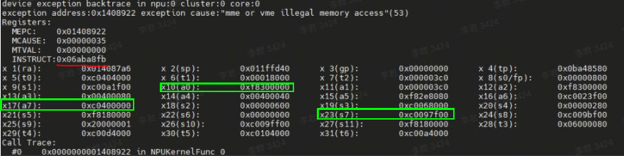
图中提示mme或vme指令访存越界,引发异常的指令编码是0x06ABe8FB(图中红色标记部分)。以现有的报错信息无法确定具体是哪条指令的问题,需手动修改CC文件来确定具体指令,过程较为繁琐,因此我们提供了一个指令编码翻译脚本工具,可直接查询具体哪条指令导致的放存越界。
指令编码翻译脚本工具(inst_decoder.py)放在MLTC安装目录下的tools下。使用脚本解析报错的指令编码,得到指令编码对应的具体指令。
运行inst_decoder.py脚本,使用--inst参数传入异常指令编码:
$ python inst_decoder.py --inst 0x06ABe8FB
isnt binary code: ['000001', '1', '01010', '10111', '1', '10', '10001', '1111011']
inst asm: veadd.mv.dimw (x17), (x23), (x10)
解析完成后直接输出编码对应的具体指令。其中inst asm: veadd.mv.dimw (x17), (x23), (x10)打印的是异常指令编码用到的是(x17),(x23),(x10)这三个指令, 根据上图中的显示信息,可得出不同指令的地址:x17=0xc0400000, x10=0xf8300000, x23=0xc0097f00,其中0xf8300000地址不在L1地址范围,可以得出x10中的地址为非法地址。
而['000001', '1', '01010', '10111', '1', '10', '10001', '1111011']打印的是指令二进制编码8个字段信息,示例如下:

参数说明:
| 参数选项 | 描述 |
|---|---|
| --inst | 异常出错的指令编码。默认值为:0x06ABE8FB。 |
在CPU上验证模型
以验证ResNet34模型为例,将通过MLTC前端转换后模型的MLIR部署到CPU上验证模型。
说明:Python接口定义请参见Python API。
-
编写Python脚本,调用MLTC的
Simulator().run()接口在CPU上部署模型,需要指定输入的mlir文件路径、运行参数,支持部署参数控制部署过程。$ cat run_resnet34_cpu.py
from mltc import Simulator
Simulator().run("resnet34.mlir", "-i data_fp32.bin -o output.bin") -
执行Python脚本。
$ python3 run_resnet34_cpu.py
推理效果演示
以YOLOv5模型为例,演示模型的编译部署,并查看NPU和CPU的推理效果,示例执行步骤如下:
-
获取官方的YOLOv5镜像以及repo。
$ git clone https://github.com/ultralytics/yolov5.git -
从HuggingFace下载pt格式的权重(
yolov5s.pt),并将权重文件移动到YOLOv5 repo所在的平级目录。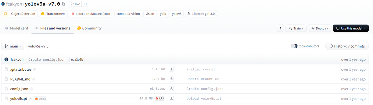
-
设置环境变量。
使用
PYTHONPATH设置YOLOv5的repo路径。$ export PYTHONPATH=~/yolov5 -
在服务器环境中安装相关python组件。
$ pip3 install torchvision==0.13.1 --index-url https://download.pytorch.org/whl/cpu
$ pip3 install opencv-python -
使用官方脚本(
export.py)将权重从pt格式转换为onnx格式。$ cd yolov5
$ python3 ./export.py --weights ../yolov5s.pt --include onnx --dynamic --opset 13 -
验证ONNX模型在CPU上的执行效果。
$ python3 ./detect.py --weights ../yolov5s.onnx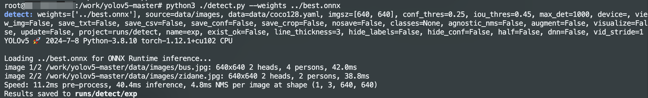
-
您可以选择将ONNX模型的metadata导出到YAML文件中。
脚本示例如下:
import onnx
import yaml

onnx_model_path = '../yolov5s.onnx'
yaml_output_path = '../yolov5s.metadata'
model = onnx.load(onnx_model_path)
metadata_dict = {prop.key: eval(prop.value) for prop in model.metadata_props}
with open(yaml_output_path, 'w') as yaml_file:
yaml.dump(metadata_dict, yaml_file, default_flow_style=False) -
编写并执行脚本,将ONNX模型转换编译为vmfb格式文件。
$ cat compile.py
from mltc import OnnxToStc
from mltc import Compiler

input_file = "../yolov5s.mlir"
output_file = "../yolov5s.vmfb"
compile_args = "-arch=npu-v1"
OnnxToStc().run("../yolov5s.onnx", input_file, "", "-i images:1x3x640x640 -s -e")
Compiler().compile(input_file, output_file, compile_args)

$ python3 compile.py -
修改部分代码适配YOLOv5的repo。
-
修改
models/common.py,修改点如下:$ git diff models/common.py
diff --git a/models/common.py b/models/common.py
index d78a8a4f..9e54b71b 100644
--- a/models/common.py
+++ b/models/common.py
@@ -472,7 +472,7 @@ class DetectMultiBackend(nn.Module):
super().__init__()
w = str(weights[0] if isinstance(weights, list) else weights)
- pt, jit, onnx, xml, engine, coreml, saved_model, pb, tflite, edgetpu, tfjs, paddle, triton = self._model_type(w)
+ pt, jit, onnx, xml, engine, coreml, saved_model, pb, tflite, edgetpu, tfjs, paddle, vmfb, triton = self._model_type(w)
fp16 &= pt or jit or onnx or engine or triton # FP16
nhwc = coreml or saved_model or pb or tflite or edgetpu # BHWC formats (vs torch BCWH)
stride = 32 # default stride
@@ -528,6 +528,9 @@ class DetectMultiBackend(nn.Module):
batch_size = batch_dim.get_length()
ov_compiled_model = core.compile_model(ov_model, device_name="AUTO") # AUTO selects best available device
stride, names = self._load_metadata(Path(w).with_suffix(".yaml")) # load metadata
+ elif vmfb:
+ from mltc import Executor
+ executor = Executor(w)
elif engine: # TensorRT
LOGGER.info(f"Loading {w} for TensorRT inference...")
import tensorrt as trt # https://developer.nvidia.com/nvidia-tensorrt-download
@@ -742,6 +745,17 @@ class DetectMultiBackend(nn.Module):
self.input_handle.copy_from_cpu(im)
self.predictor.run()
y = [self.predictor.get_output_handle(x).copy_to_cpu() for x in self.output_names]
+ elif self.vmfb:
+ def convert_dtype(type: str):
+ if "INT" in type.upper():
+ return "int32"
+ return "float16"
+ inputs = {"images": im.cpu().numpy()}
+ feeds = {}
+ for key in inputs:
+ feeds[key] = inputs[key].astype(convert_dtype(str(inputs[key].dtype)))
+ y = self.executor.run(feeds)
+ y = torch.tensor(y["output0"], dtype=torch.float32)
elif self.triton: # NVIDIA Triton Inference Server
y = self.model(im)
else: # TensorFlow (SavedModel, GraphDef, Lite, Edge TPU)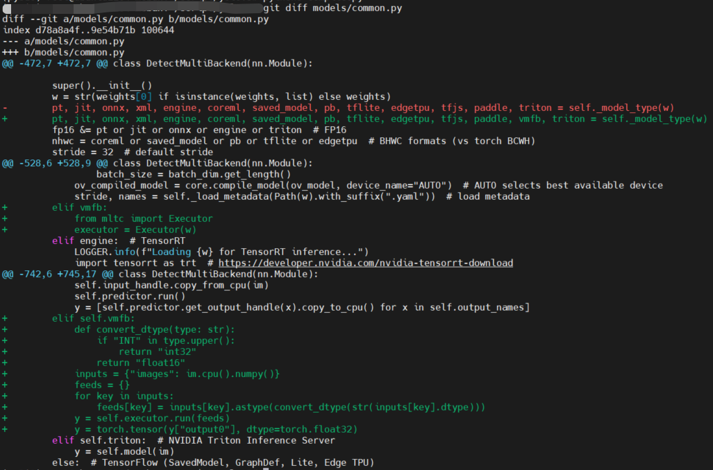
-
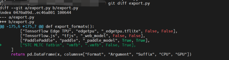
修改
export.py,修改点如下:$ git diff export.py
diff --git a/export.py b/export.py
index 0470a89d..ec46a801 100644
--- a/export.py
+++ b/export.py
@@ -175,6 +175,7 @@ def export_formats():
["TensorFlow Edge TPU", "edgetpu", "_edgetpu.tflite", False, False],
["TensorFlow.js", "tfjs", "_web_model", False, False],
["PaddlePaddle", "paddle", "_paddle_model", True, True],
+ ["STC MLTC fatbin", "vmfb", ".vmfb", False, True],
]
return pd.DataFrame(x, columns=["Format", "Argument", "Suffix", "CPU", "GPU"])
-
-
部署模型,验证模型在NPU上的执行效果。
$ python3 ./detect.py --weights ../yolov5s.vmfb --data ../yolov5s.metadata

# 忽略部分显示
image 1/2 /root/script/yolov5/data/images/bus.jpg: 640x640 4 persons, 1 bus, 28.6ms
image 2/2 /root/script/yolov5/data/images/zidane.jpg: 640x640 2 persons, 1 tie, 25.5ms
Speed: 1.0ms pre-process, 27.1ms inference, 14.5ms NMS per image at shape (1, 3, 640, 640)
Results saved to runs/detect/exp12
生成的图片示例如下:


分析推理性能
使用性能分析工具可以快速分析性能问题。性能分析工具可获取整网中算子详细的性能信息,并详细显示图调度后算子每次运行的性能信息。
性能分析工具中主要包含获取性能数据脚本:run_perf_analysis.py,脚本放在MLTC安装目录下的tools/dump_memory下,可通过mltc.__path__ 找到MLTC的安装路径。
$ python3
Python 3.10.11 (main, May 16 2023, 00:28:57) [GCC 11.2.0] on linux
Type "help", "copyright", "credits" or "license" for more information.
>>> import mltc
>>> mltc.__path__
['/root/miniconda3/envs/py310/lib/python3.10/site-packages/mltc']
>>>

$ ls /root/miniconda3/envs/py310/lib/python3.10/site-packages/mltc/tools/dump_memory
ci_compare.py  common.py  __init__.py  __pycache__  run_analysis.py  run_npu_data_analysis.py  run_perf_analysis.py  run_precision_analysis.py
使用限制
目前性能分析工具,不支持copy类算子及DMA cycle性能数据统计。具体支持的算子参见MLTC算子支持说明。
执行步骤
-
设置环境变量。
使用
DUMP_PERF_PATH设置性能数据dump后存放的目录,用于存放模型执行过程中的性能数据。# 设置性能数据存放目录
$ export DUMP_PERF_PATH=${perf_dir_name}
# 示例
$ export DUMP_PERF_PATH=~/perf_dump -
获取模型的性能数据。
运行需要性能分析的网络模型用例,具体示例可参考使用示例章节。
-
运行工具中的NPU数据分析脚本,获取节点每次运行的详细性能数据。
$ python3 run_perf_analysis.py
使用示例
将以ResNet34网络为例,使用性能分析工具获取性能数据:
$ export DUMP_PERF_PATH=~/perf_dump/resnet34_perf_dump
$ python3 compile_resnet34.py
$ python3 run_resnet34.py
$ cd /root/miniconda3/envs/py310/lib/python3.10/site-packages/mltc/tools/dump_memory
$ python3 run_perf_analysis.py
最终对比结果生成在您指定的dump数据存放目录下,即设置的DUMP_PERF_PATH下,其中包含:
-
dump_data文件夹:主要保存的是dump出来的16进制的数据。
-
result文件夹:主要保存的是最终对比分析结果。
-
skip_perf_dict.csv:执行过程中被跳过的节点以及详细跳过信息。
-
op_perf_coreid.csv:每个核上的性能数据。
-
以op_perf_0.csv性能数据为例,结果文件如下图所示:
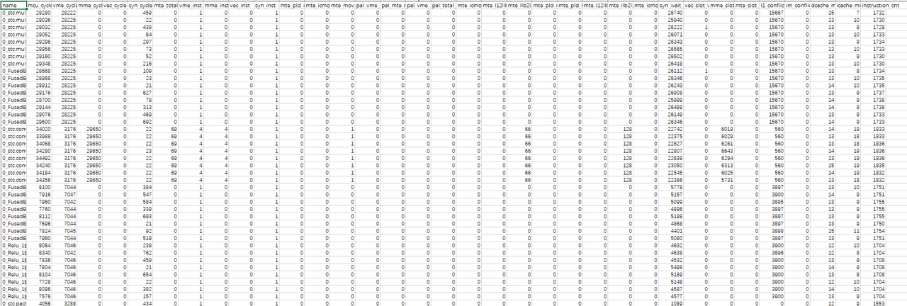
字段说明:
| 字段名 | 描述 |
|---|---|
| name | 节点名称。 |
| mcu_cycle | 总的执行周期数。 |
| vme_cycle | vme执行单元的周期数。 |
| mme_cycle | mme执行单元的周期数。 |
| vec_cycle | rvv执行单元的周期数。 |
| syn_cycle | sync执行单元的周期数。 |
| mte_total_cycle | mte总周期数。 |
| vme_inst | vme指令条数。 |
| mme_inst | mme指令条数。 |
| vec_inst | rvv指令条数。 |
| syn_inst | sync指令条数。 |
| mte_pld_inst | pld指令条数。 |
| mte_icmov_inst | icmov指令条数。 |
| mte_mov_inst | mov指令条数。 |
| pal_vme_mme_cycle | vme和mme指令并行运行周期数。 |
| pal_mte_mme_cycle | vme和mme指令并行运行周期数。 |
| pal_vme_mte_cycle | vme和mte指令并行运行周期数。 |
| pal_total_cycle | vme、mme、mte总并行运行周期数。 |
| mte_icmov_cycle | icmov指令周期数。 |
| mte_l12llb_cycle | mov_l12llb指令周期数。 |
| mte_llb2l1_cycle | mov_llb2l1指令周期数。 |
| mte_pld_cycle | pld指令周期数。 |
| mte_pld_byte | pld搬移的数据总量,字节为单位。 |
| mte_l12llb_byte | mov_l12llb搬移的数据总量,字节为单位。 |
| mte_llb2l1_byte | mov_llb2l1搬移的数据总量,字节为单位。 |
| mte_icmov_byte | icmov搬移的数据总量,字节为单位。 |
| syn_wait_cycle | syn等待的周期数。 |
| vec_slot_wait_cycle | rvv指令等待执行的周期数。 |
| mme_slot_wait_cycle | mme指令等待执行的周期数。 |
| mte_slot_wait_cycle | mte指令等待执行的周期数。 |
| l1_conflict_cycle | l1冲突周期数。 |
| im_conflict_cycle | imb冲突周期数。 |
| dcache_miss_cnt | dcache没命中次数。 |
| icache_miss_cnt | icache没命中次数。 |
| instruction_cnt | 总指令条数。 |
分析精度
使用精度分析工具可以快速定位精度问题。精度分析工具可提供生成的网络模型在CPU与NPU运行的数据对比结果分析表,还提供精度对比失败算子的详细信息,包括精度对比失败发生位置的索引号以及在CPU和NPU上的索引位置的值。
精度分析工具中主要包含以下脚本:
-
run_npu_data_analysis.py:NPU数据拼接脚本。 -
run_precision_analysis.py:NPU和CPU精度对比脚本。
所有脚本放在MLTC安装目录下的tools/dump_memory下,可通过mltc.__path__ 找到MLTC的安装路径。
$ python3
Python 3.10.11 (main, May 16 2023, 00:28:57) [GCC 11.2.0] on linux
Type "help", "copyright", "credits" or "license" for more information.
>>> import mltc
>>> mltc.__path__
['/root/miniconda3/envs/py310/lib/python3.10/site-packages/mltc']
>>>

$ ls /root/miniconda3/envs/py310/lib/python3.10/site-packages/mltc/tools/dump_memory
ci_compare.py  common.py  __init__.py  __pycache__  run_analysis.py  run_npu_data_analysis.py  run_perf_analysis.py  run_precision_analysis.py
执行步骤
-
设置环境变量。
使用
DUMP_MEMORY_PATH设置dump数据存放的目录,用于存放dump模型执行过程中的数据,基于dump数据分析出的NPU/CPU数据,以及精度对比结果。注意:该设置在运行时会影响cycle数,可通过
unset DUMP_MEMORY_PATH删除环境变量设置。# 设置dump数据存放目录
$ export DUMP_MEMORY_PATH=${dump_dir_name}
# 示例
$ export DUMP_MEMORY_PATH=~/data_dump/test_1注意:目标路径只能设置为绝对路径,且路径字符长度不超过50个字符。如果目标目录不存在,则会自动新建目录;如果目标目录已存在,则会自动删除整个目录后再自动新建。设置目录时,请多加注意。
-
获取模型的NPU数据。
编译并运行需要精度分析的网络模型用例,dump出NPU数据存放在
$DUMP_MEMORY_PATH/dump_data文件夹中对应卡的文件夹下,单卡情况下数据只会dump到0文件夹中。多卡情况下dump出来的数据会放在对应的文件夹下,下图以两卡为例,0,1文件夹下分别存放着0卡和1卡dump出来的数据。
说明:具体模型示例可参考使用示例章节。
-
获取模型的CPU数据。
编写Python脚本,调用MLTC的
Simulator().run()接口在CPU上部署模型获取dump数据。其中
--dump-dir设置的路径为DUMP_MEMORY_PATH设置的目录下cpu文件夹路径并且为绝对路径。$ cat run_resnet34_cpu.py
from mltc import Simulator
Simulator().run("resnet34.mlir", "-i data.bin -o output.bin --dump-each-op-result --dump-dir=/root/data_dump/test_1/cpu")
$ python3 run_resnet34_cpu.py -
运行工具中的NPU数据拼接脚本,对NPU数据进行拼接。
$ python3 run_npu_data_analysis.py运行后得到拼接后的NPU数据:

-
运行精度对比脚本,对比NPU和CPU数据。
$ python3 run_precision_analysis.py --ref_dtype="float32"其中,
run_precision_analysis.py脚本,运行时可传入不同参数,获取不同结果文件。您可以使用-h,--help查看帮助信息中的可选参数,其中--atol、--rtol可设置阈值、--show_graph可获取错误节点的分析图,其他参数值不建议修改。可选参数说明:
参数选项 描述 是否建议修改 -h,--help 显示帮助信息并退出。 / --ref_dtype 模型输入数据类型。 是 --cpu_dir CPU数据的存放目录。 否 --npu_dir NPU数据的存放目录。 否 --node_runtime_filename 存放每个节点的运行时刻,主要用来排序。 否 -op_config_name 每个节点的比较时候用的atol和rtol,默认是NA表示用全局的atol/rtol。特殊需求时使用。 否 --diff_cnt 最大导出的出错数据个数,默认值为128。 否 --atol 绝对误差阈值,默认值为0.005。脚本会根据绝对误差阈值的设置来统计误差超过该阈值的结果在全部结果中的占比。 是 --rtol 相对误差阈值,默认值为0.2,范围在[0.0 ~ 1.0]。脚本会根据相对误差阈值的设置来统计误差超过该阈值的结果在全部结果中的占比。 是 --show_graph 是否显示所有错误节点的分析图,取值含义: - True:显示分析图。如果数据量大,绘图会比较耗时。
- False:默认值,不显示分析图。
- op_name_diff.png :错误数据对应的绝对误差和相对误差散点图。
- op_name_diff_hist.png : 相对误差和绝对误差的直方图分布。
- op_name_hist.png:CPU和NPU数据的直方图分布。
是 --max_bins 直方图最大bin数,默认值为128。 否 --min_bins 直方图最小bin数,默认值为1,范围为[1, max_bins]。 否 --max_cores 精度分析时用到最大核数,默认值为16。 否 --map_node_dict 人为给定的参考节点与NPU节点映射dict。映射关系唯一性和正确性需得到保证。 否 --force_compare 精度分析时,是否对shape不一致但size一致的节点进行分析,默认值为False。 否
使用示例
获取精度
将以ResNet34网络为例,使用精度分析工具获取精度数据:
$ export DUMP_MEMORY_PATH=~/data_dump/test_1
$ python3 compile_resnet34.py
$ python3 run_resnet34.py
$ python3 run_resnet34_cpu.py
$ cd /root/miniconda3/envs/py310/lib/python3.10/site-packages/mltc/tools/dump_memory
$ python3 run_npu_data_analysis.py
$ python3 run_precision_analysis.py --ref_dtype="float32"
最终对比结果生成在您指定的dump数据存放目录下,即设置的DUMP_MEMORY_PATH下,其中包含:
-
cpu文件夹:主要保存的是获取网络模型在CPU上的数据。数据文件是按照实际网络模型中的节点名称来命名,将名称中的 “/” 替换成 “_”。
-
dump_data文件夹:主要保存的是dump出来的16进制的数据。经过
run_npu_data_analysis.py脚本转成二进制形式并进行数据拼接,最终输出到npu文件夹。 -
npu文件夹:主要保存的是获取网络模型在NPU上的数据,命名规则与cpu文件夹中一样。
-
result文件夹:主要保存的是最终对比分析结果。
-
skip_file_dict.csv:执行数据拼接前由于校验错误而被跳过的节点以及详细跳过信息。
-
compare_skip.log:执行CPU和NPU数据比对时被跳过的节点以及详细跳过信息。
-
cpu_vs_npu.csv:CPU和NPU数据比较结果分析表。
-
node_runtime.file:节点运行时序文件。
-
md5.csv:记录每个dump文件的md5值。
-
op_name.csv:以算子名称命名的错误算子的详细错误信息。
-
说明:结果文件具体说明可查看结果文件说明章节。
若--show_grap设为True,则在result文件夹下还会显示以算子名称命名的错误算子的分析图:
-
op_name_diff.png:错误节点对应的绝对误差和相对误差散点图。
-
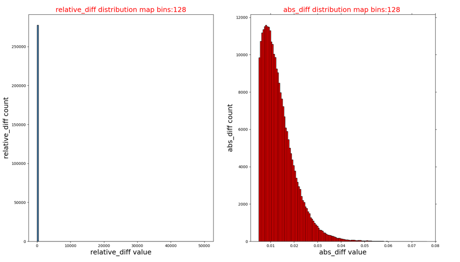
op_name_diff_hist.png:相对误差和绝对误差的直方图分布。
-
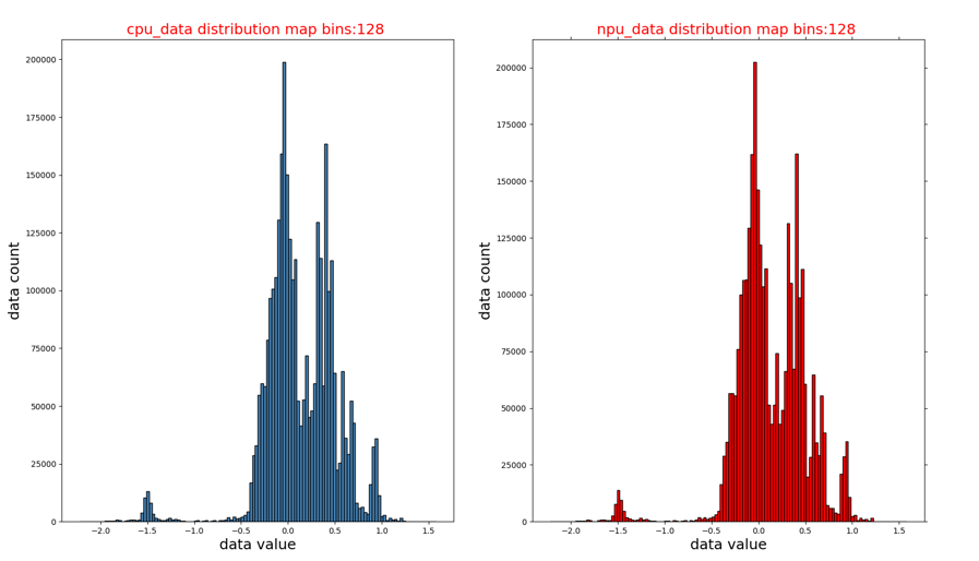
op_name_hist.png:CPU和NPU数据的直方图分布。
分析结果
按照上述步骤获取精度后,分析误差节点的精度问题。
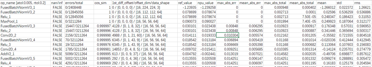
查看cpu_vs_npu.csv表中的节点误差。
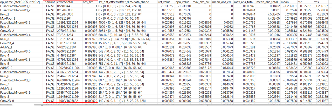
主要查看nan/inf、errors/total和cos_sim三列,分析精度问题:
-
nan/inf列有数据显示True,说明出现过NaN或inf数据,可能存在精度问题。
-
errors/total列不满足用户设置的相对误差和绝对误差的个数占比太大,可能存在现精度问题。
-
cos_sim列数值小于0.95,可能存在精度问题。
说明:每一列数据的具体说明可查看结果文件说明章节。
若遇到csv文件中无法显示完整的大批量错误数据并且是按照index排列,无法确定哪一个节点误差较大。可自行对比cpu文件夹与npu文件夹中的数据文件,分析精度误差的原因。
注意:网络模型在cpu和npu上的数据格式,数据格式可能存在NHWC或NCHW。对比时如果CPU与NPU上的数据格式不一致,需要先使用transpose函数改变数据排布。
此外,若--show_grap设为True,可查看精度对比失败节点的分析图。
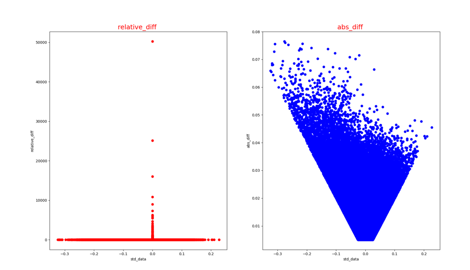
-
错误节点对应的绝对误差和相对误差散点图(op_name_diff.png):
-
CPU和NPU数据的直方图分布(op_name_hist.png):
-
相对误差和绝对误差的直方图分布(op_name_diff_hist.png):
结果文件说明
cpu_vs_npu.csv
文件描述:最终的精度对比分析结果文件。
字段说明:
| 字段名 | 描述 |
|---|---|
| op_name | 网络中节点的名称(附带显示atol/rtol参数值)。 |
| nan/inf | NPU结果数据中是否出现过nan或inf数据(比较前nan会被转成0,inf会被转成最大值)。 |
| errors/total | 不满足用户设置的相对误差和绝对误差的个数/当前算子的总个数(单位:个)。 |
| cos_sim | NPU结果和CPU结果的余弦相似度,数据越大越好。 |
| 1st_diff_offset/offset_dim/data_shape | 第一个数据错误的位置,对应的维度信息,数据shape信息。 |
| ref_value | 标准模型(TensorFlow模型、ONNX模型)第一个发生错误时的数据(目前仅保留小数点后6位有效数字),若当前算子均未发生精度对比失败,此时的值为算子输出的第一个数据。 |
| npu_value | 基于九章NPU框架的推理模型,第一个发生错误时的数据(目前仅保留小数点后6位有效数字),若当前算子均未发生精度对比失败,此时的值为算子输出的第一个数据。 |
| max_abs_err | 节点错误数据的最大绝对误差。 |
| mean_abs_err | 节点错误数据的平均绝对误差。 |
| max_abs_total | 节点数据的最大相对误差。 |
| mean_abs_total | 节点数据的平均相对误差。 |
| mean | 参考数据(TensorFlow模型、ONNX模型的数据)的均值。 |
| std | 参考数据(TensorFlow模型、ONNX模型的数据)的方差。 |
| rms | 参考数据(TensorFlow模型、ONNX模型的数据)的均方根值(root mean square)。 |
op_name.csv
文件描述:精度对比失败算子详细信息。

字段说明:
| 字段名 | 说明 |
|---|---|
| index | 精度对比失败发生的索引号。 |
| std_value | 标准模型相应索引位置的值。 |
| npu_value | 九章NPU模型相应索引位置的值。 |
| abs_diff | 绝对误差。 |
| relative_diff | 相对误差。 |
误差类型及判断方法
NPU每个节点计算输出的误差可以分为两类:
-
计算错误:由硬件或软件Bug问题导致的错误。
-
累积精度误差:由于在NPU上采用FP16计算,相对于CPU上使用FP32计算存在精度损失,并且这个精度损失逐层累积造成的误差。
其他精度问题
-
CPU与NPU输出结果均存在NaN。
当发现CPU与NPU运行出来的结果都存在NaN的问题时,可考虑网络模型本身的问题,可能存在模型中算子的参数不合法的情况。
-
可能是算子参数为inf,使得与其他数字相乘会出错,导致结果都是NaN,此时应考虑算子问题。
-
可能是模型输入不合适,例如输入中包含负数,而网络模型中存在Log这一类的算子,经过该节点是会出现计算错误,使得CPU和NPU的运行结果为NaN。
-
CPU输出正常而NPU结果为NaN。
当发现CPU的输出正常而NPU运行出来的结果为NaN的问题时,可考虑是算子参数导致,其表现是中间输出结果超FP16范围(65504),通常两个大数相乘或者除以一个极小的数时容易出现结果超出FP16范围问题(65504)。
精度分析定位技巧
-
随机精度问题定位
如果网络存在随机精度问题且在打开Dump Memory功能时也存在随机问题的情况下,可以用以下方法定位:
将模型网络运行两遍,数据分别dump在两个不同的路径下,然后分别运行
run_npu_data_analysis.py脚本,在脚本运行过程中,运行完下图中第一个进度条后就可停止,工具会计算每个dump文件的md5并记录在result/md5.csv文件中。
比较两个dump路径下的
result/md5.csv文件就能知道那个节点的输出存在随机问题。此外可以观察md5值是否是变化,来判断网络是否存在随机精度问题。

-
不跑stc-run进行精度分析
在修改过程中可能会引入一些问题导致之前精度正确的网络出现精度错误问题,则可以通过以下方法加速定位:
-
分别获取精度正确和精度错误的网络的NPU上的数据,dump数据后使用
run_npu_data_analysis.py脚本完成数据拼接。 -
将精度正确的网络Dump出来的放在npu文件夹下的所有NPU数据文件,拷贝到精度错误网络的cpu文件夹下,作为参考数据进行对比。
-
使用
run_precision_analysis.py脚本对比数据。
相比跑stc-run的优势在于,参考结果也是由NPU运行获取的,精度对比数据差异几乎没有,进而避免了查看精度分析结果时考虑FP16累加引入的不确定性。
-
-
出现精度问题时,可以考虑查看
STC_SET_DEVICES指定的Cluster数。首根轴会根据Cluster数进行切分补Pad操作,但部分模型或算子不可切分,切分后会出现精度问题。所以若模型无batch或者batch轴不可切分的情况,可尝试使用
STC_SET_DEVICES指定单个Cluster进行运行部署。
常见问题
-
stc-run运行失败问题
目前stc-run支持的算子及支持的数据类型并不完善,在跑stc-run时可能遇到folder失败问题,正在完善修复中。
-
重复/丢失节点问题
-
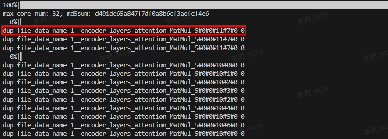
重复节点问题:
PASS在Span传递过程中各种原因导致Span重名问题,导致dump出来的节点名称出现重复的现象,工具在分析过程中会报以下错误:
-
丢失节点问题:
节点名重复导致信息不一致,会出现节点丢失的现象,工具在分析过程中中会报以下错误:
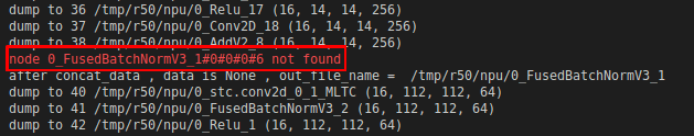
上述两个节点问题的错误日志会记录在
result/skip_file_dict.csv,如下所示:
-
-
多轮运行导致伪重复节点问题
在获取大模型数据时只能跑单轮,多轮运行会导致Span重复问题。查看数据如何区分是不是多轮dump导致,可以通过以下方式,如果文件数多于1个,说明是跑多轮导致。
$ ls dump_data/0/0_map_name@0.*
dump_data/0/0_map_name@0.011fda60_000001d2.dat dump_data/0/0_map_name@0.013fda60_000001d2.dat -
不支持dump的算子
数据拷贝类算子暂不支持dump功能,例如slice/concat/split等算子。
生成量化模型
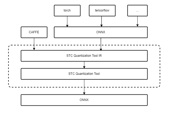
SNQ量化工具可以对小模型进行PTQ量化,量化工具能够直接支持的模型格式有ONNX、CAFFE,其他模型格式需先转成ONNX。若有PyTorch大模型量化需求,可选择使用SNC量化工具,详情可参见STC_LLM使用指南。
说明:如果在GPU上使用工具,请安装CUDA 11.8版本、CUDA驱动(cuda-repo-ubuntu2004-12-1-local_12.1.0-530.30.02-1_amd64.deb)以及显卡。
执行步骤
以Bert128模型为例演示执行步骤:
-
配置YAML文件。
根据网络的不同填写模型运行的基本参数,如果模型不是ONNX格式的需要做模型转换,内部提供了pb与pth模型的转化。量化策略与精度校准可以根据模型验证结果自行调节,找到合适当前网络的策略。
以下是Bert128模型的YAML文件:
# ----------------------------------------------------------
# 模型运行基本参数
# ----------------------------------------------------------

model_name: "bert_128"
local_model_path: "./bert_128_tf.onnx"
input_name: ["embedding_lookup:0","input_mask:0","one_hot:0"]
input_shape: [[1024,768],[8,1,128],[1024,2]]
input_dtype: ["torch.float32", "torch.float32", "torch.float32"]
batch_size: 64
output_node: "loss/Softmax:0"
# ----------------------------------------------------------
# 模型转为onnx
# ----------------------------------------------------------

# 是否需要转化为ONNX模型,True:若输入模型不是onnx,需要转换 False:不需要转换
is_translate: False
# 提供两种模型的转换:pb, pth
model_type: "onnx"
onnx_target_file: "./bert_128.onnx"

# ----------------------------------------------------------
# 模型输入数据
# ----------------------------------------------------------

# 输入是否已经经过预处理,True: 已经过预处理,可从本地直接读取, False: 未经过预处理,需要添加预处理函数,返回模型输入数据
input_preprocess: False
# 已预处理后的数据,可以直接输入模型运行
# 提供两种文件读取:npy, bin
# 默认文件命名格式:file_path+file_name+index+file_type
#                 ./bert128_datasets/embedding_look_up_0.npy
dataset:
      file_type: "npy"
      file_path: "./bert128_dataset/"
      file_name: ["embedding_lookup_","input_mask_","one_hot_"]

# 未预处理的数据,请修改预处理脚本文件,提供校准数据,8-256组即可
# def pre_process(config:dict, data_num:int) -> List[{inputname_0:tensor,inputname_1:tensor},...]:
#    ...
# 预处理脚本文件名
pre_process: "pre_process"
file_list: []

# ----------------------------------------------------------
# 量化策略, 目前在NPUv1上可以改动的有限
# ----------------------------------------------------------

# 量化总开关
do_quantize: true
target_file: "./bert128_quant.onnx"

# 参数可选项:
#        calibrate: kl, minmax, percentile, mse
#        round: ROUND_TOWARDS_ZERO, ROUND_HALF_EVEN
#        policy: PerTensor, PerChannel
#        # 按照哪个轴做per_channel 开启PerChannel时需要指定,PerTensor不可包含这条属性
#        channel_axis: -2, -1, 0, 1
#        Symmetric: true, false(open asymmetric)
conv:
  activation:
    calibrate: "kl"
    round: "ROUND_TOWARDS_ZERO"
    policy: "PerTensor"
    Symmetric: true
  parameter:
    calibrate: "minmax"
    round: "ROUND_HALF_EVEN"
    policy: "PerChannel"
    Symmetric: true
    channel_axis: 0

matmul:
  activation:
    calibrate: "kl"
    round: "ROUND_TOWARDS_ZERO"
    policy: "PerTensor"
    Symmetric: true
  parameter:
    calibrate: "minmax"
    round: "ROUND_HALF_EVEN"
    policy: "PerChannel"
    Symmetric: true
    channel_axis: 1

# ----------------------------------------------------------
# 量化精度校准选项,不改变量化策略的情况下,主要通过关闭量化误差
# 较大的算子来提高精度
# ----------------------------------------------------------

# 总开关————是否开启关闭算子来提高量化精度
close_op: true
# 关闭误差最大的算子数量
close_op_num: 0
# 关闭量化精度小于阈值的所有算子,close_op_num为0时生效
close_value: 0.999
# 关闭指定算子,填入算子名称
close_op_name: []

# 寻找最优激活校准方式
activate_calib_algo: false

# ----------------------------------------------------------
# 模型精度验证方式
# ----------------------------------------------------------

# SNQ验证模型精度标志,开启时不进行激活函数————gelu融合
test_flag: true
# 验证模型精度脚本
# def quantonnxrun(config:dict):
#    ...
# 验证模型精度脚本文件名
test_run: test_run
# 验证数据组数
test_num: 5
atol: 0.04
rtol: 0.01

# 模型运行设备(cpu、cuda)
device: cpu
输入数据如果未经过预处理,需要添加预处理函数,并在YAML文件中标明预处理脚本。Bert128的预处理脚本可参考代码示例中的
pre_process.py。已经做好了预处理的数据不一定适合所有场景,所以为了量化效果更加完善,建议用户选取自己需要的校准集来进行网络量化。# 输入是否已经经过预处理,true: 已经过预处理,可从本地直接读取, False: 未经过预处理,需要添加预处理函数,返回模型输入数据
input_preprocess: False
# 已预处理后的数据,可以直接输入模型运行
# 提供两种文件读取:npy, bin
# 默认文件命名格式:file_path+file_name+index+file_type
# ./bert128_datasets/embedding_look_up_0.npy
dataset:
file_type: "npy"
file_path: "./bert128_dataset/"
file_name: ["embedding_lookup_","input_mask_","one_hot_"]
# 未预处理的数据,请修改预处理脚本文件,提供校准数据,8-256组即可
# def pre_process(config:dict, data_num:int) -> List[{inputname_0:tensor,inputname_1:tensor},...]:
# ...
# 预处理脚本文件名
pre_process: "pre_process"
file_list: []对精度有要求的模型,可接入结构的后处理,添加结果对比代码,并在YAML文件中标明预处理脚本。Bert128的验证模型精度脚本可参考代码示例中的
test_tun.py。原始模型与量化后的模型都会运行,可对它们的结果进行比较,得到精度对比结果。不同网络的验证模型精度脚本需要根据用户自己对网络的结果评判标准自己构建代码。
说明:测试模块使用的是ONNX Runtime运行,不能含有ONNX Runtime无法运行的算子。
# ----------------------------------------------------------
# 模型精度验证方式
# ----------------------------------------------------------

# SNQ验证模型精度标志,开启时不进行激活函数————gelu融合
test_flag: true
# 验证模型精度脚本
# def quantonnxrun(config:dict):
#    ...
# 验证模型精度脚本文件名
test_run: test_run
# 验证数据组数
test_num: 5
atol: 0.04
rtol: 0.01
说明:配置的YMAL文件、数据预处理脚本和验证精度脚本需放在同一目录下。
-
启动量化命令,生成量化后模型和模型参数。
$ cd bert128
$ ls
bert128_dataset  bert_128_tf.onnx  default_config.yaml  pre_process.py  test_run.py
$ auto_quant --config default_config.yaml -
将量化后的模型和分离的模型参数一起放到NPU上使用MLTC编译运行。具体编译运行方式可参考在NPU上部署模型章节。
代码示例
Bert128模型预处理脚本(pre_process.py),请自行准备好Bert128的数据集和Bert128的ONNX模型。
import torch
import numpy as np
import os
from minio import Minio
from stcnq.utilities.utils import pull_from_minio

def pre_process(config: dict, data_num: int = 64) -> list:
    """model preprocessed data

    Args:
        filelist (list, optional): input file list. Defaults to [].
        data_num (int, optional): output data number.  Return the number of date.

    Returns:
        dict: model input data
    """

    result = []
    # code ...
    current_dir = config["local_model_path"]
    BATCH_SIZE = data_num
    INPUT_NAME = config["input_name"]

    if config["dataset"]["file_type"] == "npy":
        result = [
            {
                INPUT_NAME[x]: torch.from_numpy(
                    np.load(config["dataset"]["file_path"] + config["dataset"]["file_name"][x] + str(idx) + ".npy")
                ).to(torch.float32)
                for x in range(len(INPUT_NAME))
            }
            for idx in range(BATCH_SIZE)
        ]
    elif config["dataset"]["file_type"] == "bin":
        result = [
            {
                INPUT_NAME[x]: torch.load(
                    np.load(config["dataset"]["file_path"] + config["dataset"]["file_name"][x] + str(idx) + ".bin")
                ).to(torch.float32)
                for x in range(len(INPUT_NAME))
            }
            for idx in range(BATCH_SIZE)
        ]
    else:
        raise ("not support data  file type")
    """result type

    Returns:
        result = [
            {
                "input_name1": data1,
                "input_name2": data2
            },
            {
                "input_name1": data3,
                "input_name2": data4
            },...
        ]
    data type-----> tensor of torch
    """
    config["input_preprocess"] = True
    return result
Bert128模型验证精度脚本(test_run.py)
import onnxruntime
import torch
import os
import math
import numpy as np
import importlib
import torch.nn.functional as Fun
import matplotlib.pyplot as plt

def compare(result, ref, atol=0.005, rtol=2, accumulate=1):
    """compare"""
    if len(result) != len(ref):
        raise RuntimeError(f"result length:{len(result)} is not equal to gold data length: {len(ref)}")
    atol = max(atol, atol / 50 * accumulate)
    rtol = int(rtol * np.sqrt(accumulate * 2))
    # print(f"Comparing result using atol={atol}, rtol={rtol}")

    result_int = np.copy(result)
    result_int.dtype = "int16"
    ref_int = np.copy(ref)
    ref_int.dtype = "int16"

    mismatch = 0
    max_abs_diff = 0.0
    max_rel_diff = 0
    abs_diff_list = []
    rel_diff_list = []

    all_mismatch = []
    for i, _ in enumerate(result):
        abs_diff = abs(result[i] - ref[i])
        rel_diff = abs(result_int[i] - ref_int[i])
        abs_diff_list.append(abs_diff)
        rel_diff_list.append(rel_diff)
        if abs_diff > max_abs_diff:
            max_abs_diff = abs_diff
        if rel_diff > max_rel_diff:
            max_rel_diff = rel_diff
        if abs_diff > atol and rel_diff > rtol:
            all_mismatch.append((i, abs_diff, rel_diff))
            mismatch += 1

    # if len(abs_diff_list) > 0:
    #     print("mean absolute diff: {}".format(sum(abs_diff_list) / len(abs_diff_list)))
    # else:
    #     print("mean absolute diff: 0.0")
    # if len(rel_diff_list) > 0:
    #     print("mean relative diff: {}".format(sum(rel_diff_list) / len(rel_diff_list)))
    # else:
    #     print("mean relative diff: 0.0")
    if mismatch != 0:
        # print(
        #     f"Failed: {mismatch}/{len(result)} mismatch,"
        #     f"max absolute diff: {max_abs_diff}, max relative diff: {max_rel_diff}"
        # )
        n = min(10, mismatch)

        def show_mismatch(n, idx, msg):
            mismatches = sorted(all_mismatch, key=lambda x: x[idx], reverse=True)[:n]
            for item in mismatches:
                i = item[0]
                # print(
                #     f"{msg} mismatch: out[{i}] = {result[i]}({result_int[i]}),"
                #     f"ref[{i}] = {ref[i]}({ref_int[i]}), atol={item[1]}, rtol={item[2]}",
                #     flush=True,
                # )

        # print(f"n---------- top {n} max abs mismatches ----------")
        show_mismatch(n, 1, "abs")
        # print(f"n---------- top {n} max rel mismatches ----------")
        show_mismatch(n, 2, "rel")
        return False
    # print(
    #     f"Success: {mismatch}/{len(result)} mismatch,"
    #     f"max absolute diff: {max_abs_diff}, max relative diff: {max_rel_diff}"
    # )
    # print("Succeed")
    return True

def result_process(test_num, label_path, tf_position_path, tf_prob_path):
    label = np.loadtxt(label_path)
    tc = np.loadtxt("./model_zoo/quant_argmax.txt")
    tc_prob = np.loadtxt("./model_zoo/quant_prob.txt")
    tf = np.loadtxt(tf_position_path)
    tf_prob = np.loadtxt(tf_prob_path)
    equal_size = 0
    for i in range(0, test_num):
        if label[i] == tc[i]:
            equal_size += 1
    print("tc true_label_accuracy: ", equal_size, equal_size / test_num)
    equal_size = 0
    for i in range(0, test_num):
        if label[i] == tf[i]:
            equal_size += 1
    print("tf true_label_accuracy: ", equal_size, equal_size / test_num)
    # tf_label_accuracy
    equal_size = 0
    for i in range(0, test_num):
        if tf[i] == tc[i]:
            equal_size += 1
    print("tf_label_accuracy: ", equal_size, equal_size / test_num)
    # max_abs_diff
    max_diff = 0
    total_diff = 0
    abs_diff_list = []
    for i in range(0, test_num):
        cur_diff = abs(tf_prob[i][int(tf[i])] - tc_prob[i][int(tf[i])])
        abs_diff_list.append(cur_diff)
        total_diff += cur_diff
        if cur_diff > max_diff:
            max_diff = cur_diff
    print("max_abs_diff: ", max_diff)
    # mean_abs_diff
    mean_diff = total_diff / test_num
    print("mean_abs_diff: ", mean_diff)

    plt.hist(abs_diff_list, bins=100, density=False, histtype="bar")
    plt.title("Histogram of absolute error, samples 10570")
    plt.savefig("cmp.png")
    # std_abs_diff
    acc_diff = 0
    for i in range(0, test_num):
        cur_diff = abs(tf_prob[i][int(tf[i])] - tc_prob[i][int(tf[i])])
        std_diff = (cur_diff - mean_diff) * (cur_diff - mean_diff)
        acc_diff += std_diff
    print("std_abs_diff: ", math.sqrt(acc_diff) / (test_num - 1))
    # max_rel_diff
    tf_prob_int = np.copy(tf_prob)
    tf_prob_int.dtype = "int16"
    tc_prob_int = np.copy(tc_prob)
    tc_prob_int.dtype = "int16"

    total_rel_diff = 0
    max_rel_diff = 0
    for i in range(0, test_num):
        cur_rel_diff = abs(int(tf_prob_int[i][int(tf[i])]) - int(tc_prob_int[i][int(tf[i])]))
        total_rel_diff += cur_rel_diff
        if cur_rel_diff > max_rel_diff:
            max_rel_diff = cur_rel_diff
    print("max_rel_diff: ", max_rel_diff)

    # mean_rel_diff
    mean_rel_diff = total_rel_diff / test_num
    print("mean_rel_diff: ", mean_rel_diff)
    # std _rel_diff
    acc_rel_diff = 0
    for i in range(0, test_num):
        cur_rel_diff = abs(int(tf_prob_int[i][int(tf[i])]) - int(tc_prob_int[i][int(tf[i])]))
        std_rel_diff = (cur_rel_diff - mean_rel_diff) * (cur_rel_diff - mean_rel_diff)
        acc_rel_diff += std_rel_diff
    print("std_rel_diff: ", math.sqrt(acc_rel_diff) / (test_num - 1))

def quantonnxrun(config: dict):
    module_name = config["pre_process"]
    module = importlib.import_module(module_name)
    pre_process = getattr(module, "pre_process")
    test_num = config["test_num"]
    input_name = config["input_name"]
    if config["input_preprocess"]:
        if config["dataset"]["file_type"] == "npy":
            dataset = [
                {
                    input_name[x]: np.load(
                        config["dataset"]["file_path"] + config["dataset"]["file_name"][x] + str(idx) + ".npy"
                    ).astype(np.float32)
                    for x in range(len(input_name))
                }
                for idx in range(test_num)
            ]
        elif config["dataset"]["file_type"] == "bin":
            dataset = [
                {
                    input_name[x]: np.load(
                        config["dataset"]["file_path"] + config["dataset"]["file_name"][x] + str(idx) + ".bin"
                    ).astype(np.float32)
                    for x in range(len(input_name))
                }
                for idx in range(test_num)
            ]
        else:
            raise ("not support data  file type")
    else:
        dataset = pre_process(config, test_num)

        for idx in range(test_num):
            for x in range(len(input_name)):
                if not torch.is_tensor(dataset[idx][input_name[x]]):
                    raise TypeError("data type is not torch")
                else:
                    dataset[idx][input_name[x]] = dataset[idx][input_name[x]].numpy()
    onnx_run = onnxruntime.InferenceSession(config["local_model_path"], providers=onnxruntime.get_available_providers())
    onnx_outputs = [onnx_run.run([config["output_node"]], dataset[idx]) for idx in range(test_num)]

    quant_run = onnxruntime.InferenceSession(config["target_file"], providers=onnxruntime.get_available_providers())
    quant_outputs = [quant_run.run([config["output_node"]], dataset[idx]) for idx in range(test_num)]

    # you can modify the following code to achieve accuracy comparison
    pass_count = 0
    pos_count = 0
    for idx in range(test_num):
        golden = onnx_outputs[idx][0]
        quant = quant_outputs[idx][0]
        position_quant = np.argmax(quant, axis=1)
        position_golden = np.argmax(golden, axis=1)
        for x in range(8):
            ret = compare(quant[x], golden[x], atol=config["atol"], rtol=config["rtol"])
            if ret:
                pass_count += 1
            if position_golden[x] == position_quant[x]:
                pos_count += 1

        print("quant::", idx, quant)
        print("golden::", idx, golden)
    print("pass_count:", pass_count, "t pass_rate:", "%.2f%%" % (pass_count / (8 * test_num) * 100))
    print("position_count:", pos_count, "t pass_rate:", "%.2f%%" % (pos_count / (8 * test_num) * 100))
图分组性能调优
为解决部分模型因自动分组导致的性能不佳问题,我们开发了手动图分组工具。该工具允许用户在MLTC编译过程中,通过提供图分组配置文件,指导编译器执行特定的分组切分操作。Manual Group Partition功能通过手动配置--manual-partition-file编译选项的方式指导MLTC对模型进行优化,具体涵盖 group切分、LLB切分、多核切分与L1切分。
Compiler().compile(input_file, output_file, "-arch=npu-v1 --manual-partition-file=/home/resnet50.yml")
以ResNet50量化模型为例,演示手动图分组工具的操作步骤:
-
获取可视化IR。
在进行手动Group Partition前需一份可视化的IR,该IR不能直接使用原始模型的IR,原因在于编译过程会做一些算子拆分、替换等操作,这些操作会引起IR中的span发生变化进而导致group切分的span无法对应。可通过运行
slim.py脚本获取正确的可视化IR。$ python slim.py --mlir_path /root/script/resnet50/resnet50.mlir --out_path resnet50_view.mlir其中脚本放在MLTC安装目录下的
tools下,可通过mltc.__path__找到MLTC的安装路径。可选参数说明:
参数选项 描述 是否必选 --mlir_path 模型原始的MLIR的完整路径。 是 --out_path 可视化MLIR输出的完整路径。 是 --max_cores 处理过程中使用的最大线程数。 否 脚本会dump出group partition前一个IR作为待处理的中间IR。对该中间IR做如下处理后输出可视化IR:
-
将const value全部显示成
value = dense_resource<__elided__>以减少可视化MLIR文件大小。 -
只保留可视化需要的span attr。
-
删除和替换Netron不支持的信息。例如,删除
builtin.module信息;将func.func"()替换成"func.func"@NPUKernelFunc() {等。
-
-
使用Netron工具打开可视化IR,根据可视化IR性能调优。group是一个多输入、单输出的DAG,可以描述整个计算图中的一个子图。图分组切分只针对group。
-
配置YAML文件进行手动图分组。
配置文件字段包含:
-
一级字段
字段名 类型 含义 groups Array < Group > 包含所有分组信息的标志。 -
二级字段
Group用以描述具体的分组信息,从属于一级字段groups。
字段名 类型 含义 inputs Array < String > 输入节点的span name。 output String 输出节点的span name。 split_axis Array < int64_t > 当前group的切分轴。 split_factor Array < int64_t > 当前group的切分份数。 配置文件要求:
-
配置文件路径必须有效且可访问。
-
配置文件必须包含
groups字段。 -
每个 group 必须包含
inputs、output、split_axis、split_factor二级字段。 -
split_axis与split_factor字段的长度必须相同。 -
inputs字段中的span name必须是有效的。 -
output字段中的span name必须是有效的。 -
不同 group 的
output字段值不能重复。 -
inputs中的每个span name必须是某个group的output,或block argument的user。
配置文件示例:
# Array<Group>
groups:
  # Group 0
  - inputs: ["bn_data_FusedBatchNorm_1_mul_4/0"]
    output: "PPQ_Operation_24_quantize_0/47"
    split_axes: [0]
    split_factors: [8]
  # Group 1
  - inputs: ["PPQ_Operation_24_quantize_0/47"]
    output: "PPQ_Operation_63_quantize_0/104"
    split_axes: [0]
    split_factors: [4]
  # Group 2
  - inputs: ["PPQ_Operation_63_quantize_0/104"]
    output: "PPQ_Operation_117_quantize_0/188"
    split_axes: [0]
    split_factors: [2]
  # Group 3
  - inputs: ["PPQ_Operation_117_quantize_0/188"]
    output: "softmax_Softmax_div_4/242"
    split_axes: [0]
split_factors: [1] -
-
编译模型。
配置
--manual-partition-file编译选项编译模型,指导MLTC对模型进行优化。$ cat compile_resnet50.py
from mltc import Compiler
# 输入mlir文件路径
input_file = "resnet50_view.mlir"
# 输出vmfb文件路径
output_file = "resnet50_stc.vmfb"
# 编译参数
compile_args = "-arch=npu-v1 --manual-partition-file=/home/resnet50.yml"
Compiler().compile(input_file, output_file, compile_args)